Гетероскедастичность
Случайной ошибкой
называется отклонение в линейной модели
множественной регрессии:
εi=yi–β0–β1x1i–…–βmxmi
В связи с тем, что
величина случайной ошибки модели
регрессии является неизвестной величиной,
рассчитывается выборочная оценка
случайной ошибки модели регрессии по
формуле:
![]()
где ei – остатки
модели регрессии.
Термин
гетероскедастичность в широком смысле
понимается как предположение о дисперсии
случайных ошибок модели регрессии.
При построении
нормальной линейной модели регрессии
учитываются следующие условия, касающиеся
случайной ошибки модели регрессии:
6) математическое
ожидание случайной ошибки модели
регрессии равно нулю во всех наблюдениях:
![]()
7) дисперсия случайной
ошибки модели регрессии постоянна для
всех наблюдений:
![]()
 между значениями
случайных ошибок модели регрессии в
любых двух наблюдениях отсутствует
систематическая взаимосвязь, т. е.
случайные ошибки модели регрессии не
коррелированны между собой (ковариация
случайных ошибок любых двух разных
наблюдений равна нулю):
![]()
Второе условие
![]()
означает
гомоскедастичность (homoscedasticity – однородный
разброс) дисперсий случайных ошибок
модели регрессии.
Под гомоскедастичностью
понимается предположение о том, что
дисперсия случайной ошибки βi является
известной постоянной величиной для
всех наблюдений.
Но на практике
предположение о гомоскедастичности
случайной ошибки βi или остатков модели
регрессии ei выполняется не всегда.
Под гетероскедастичностью
(heteroscedasticity – неоднородный разброс)
понимается предположение о том, что
дисперсии случайных ошибок являются
разными величинами для всех наблюдений,
что означает нарушение второго условия
нормальной линейной модели множественной
регрессии:
![]()
Гетероскедастичность
можно записать через ковариационную
матрицу случайных ошибок модели
регрессии:

Тогда можно
утверждать, что случайная ошибка модели
регрессии βi подчиняется нормальному
закону распределения с нулевым
математическим ожиданием и дисперсией
G2Ω:
εi~N(0; G2Ω),
где Ω – матрица
ковариаций случайной ошибки.
Если дисперсии
случайных ошибок
![]()
модели регрессии
известны заранее, то проблема
гетероскедастичности легко устраняется.
Однако в большинстве случаев неизвестными
являются не только дисперсии случайных
ошибок, но и сама функция регрессионной
зависимости y=f(x), которую предстоит
построить и оценить.
Для обнаружения
гетероскедастичности остатков модели
регрессии необходимо провести их анализ.
При этом проверяются следующие гипотезы.
Основная гипотеза
H0 предполагает постоянство дисперсий
случайных ошибок модели регрессии, т.
е. присутствие в модели условия
гомоскедастичности:
![]()
Альтернативная
гипотеза H1 предполагает непостоянство
дисперсиий случайных ошибок в различных
наблюдениях, т. е. присутствие в модели
условия гетероскедастичности:
![]()
Гетероскедастичность
остатков модели регрессии может привести
к негативным последствиям:
1) оценки неизвестных
коэффициентов нормальной линейной
модели регрессии являются несмещёнными
и состоятельными, но при этом теряется
свойство эффективности;
2) существует большая
вероятность того, что оценки стандартных
ошибок коэффициентов модели регрессии
будут рассчитаны неверно, что конечном
итоге может привести к утверждению
неверной гипотезы о значимости
коэффициентов регрессии и значимости
модели регрессии в целом.
Гомоскедастичность
Гомоскедастичность
остатков означает, что дисперсия каждого
отклонения одинакова для всех значений
x. Если это условие не соблюдается, то
имеет место гетероскедастичность.
Наличие гетероскедастичности можно
наглядно видеть из поля корреляции.


Т.к. дисперсия
характеризует отклонение то из рисунков
видно, что в первом случае дисперсия
остатков растет по мере увеличения x, а
во втором – дисперсия остатков достигает
максимальной величины при средних
значениях величины x и уменьшается при
минимальных и максимальных значениях
x. Наличие гетероскедастичности будет
сказываться на уменьшении эффективности
оценок параметров уравнения регрессии.
Наличие гомоскедастичности или
гетероскедастичности можно определять
также по графику зависимости остатков
от теоретических значений
![]() .
.

Соседние файлы в предмете [НЕСОРТИРОВАННОЕ]
- #
- #
- #
- #
- #
- #
- #
- #
- #
- #
- #
From Wikipedia, the free encyclopedia
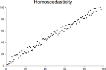
Plot with random data showing homoscedasticity: at each value of x, the y-value of the dots has about the same variance.
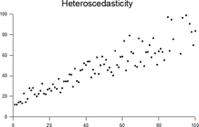
Plot with random data showing heteroscedasticity: The variance of the y-values of the dots increase with increasing values of x.
In statistics, a sequence (or a vector) of random variables is homoscedastic () if all its random variables have the same finite variance. This is also known as homogeneity of variance. The complementary notion is called heteroscedasticity. The spellings homoskedasticity and heteroskedasticity are also frequently used.[1][2][3]
Assuming a variable is homoscedastic when in reality it is heteroscedastic () results in unbiased but inefficient point estimates and in biased estimates of standard errors, and may result in overestimating the goodness of fit as measured by the Pearson coefficient.
The existence of heteroscedasticity is a major concern in regression analysis and the analysis of variance, as it invalidates statistical tests of significance that assume that the modelling errors all have the same variance. While the ordinary least squares estimator is still unbiased in the presence of heteroscedasticity, it is inefficient and generalized least squares should be used instead.[4][5]
Because heteroscedasticity concerns expectations of the second moment of the errors, its presence is referred to as misspecification of the second order.[6]
The econometrician Robert Engle was awarded the 2003 Nobel Memorial Prize for Economics for his studies on regression analysis in the presence of heteroscedasticity, which led to his formulation of the autoregressive conditional heteroscedasticity (ARCH) modeling technique.[7]
Definition[edit]
Consider the linear regression equation 


More generally, if the variance-covariance matrix of disturbance

Examples[edit]
Heteroscedasticity often occurs when there is a large difference among the sizes of the observations.
- A classic example of heteroscedasticity is that of income versus expenditure on meals. As one’s income increases, the variability of food consumption will increase. A poorer person will spend a rather constant amount by always eating inexpensive food; a wealthier person may occasionally buy inexpensive food and at other times eat expensive meals. Those with higher incomes display a greater variability of food consumption.
- Imagine you are watching a rocket take off nearby and measuring the distance it has travelled once each second. In the first couple of seconds your measurements may be accurate to the nearest centimeter, say. However, 5 minutes later as the rocket recedes into space, the accuracy of your measurements may only be good to 100 m, because of the increased distance, atmospheric distortion and a variety of other factors. The data you collect would exhibit heteroscedasticity.
Consequences of heteroscedasticity[edit]
One of the assumptions of the classical linear regression model is that there is no heteroscedasticity. Breaking this assumption means that the Gauss–Markov theorem does not apply, meaning that OLS estimators are not the Best Linear Unbiased Estimators (BLUE) and their variance is not the lowest of all other unbiased estimators.
Heteroscedasticity does not cause ordinary least squares coefficient estimates to be biased, although it can cause ordinary least squares estimates of the variance (and, thus, standard errors) of the coefficients to be biased, possibly above or below the true of population variance. Thus, regression analysis using heteroscedastic data will still provide an unbiased estimate for the relationship between the predictor variable and the outcome, but standard errors and therefore inferences obtained from data analysis are suspect. Biased standard errors lead to biased inference, so results of hypothesis tests are possibly wrong. For example, if OLS is performed on a heteroscedastic data set, yielding biased standard error estimation, a researcher might fail to reject a null hypothesis at a given significance level, when that null hypothesis was actually uncharacteristic of the actual population (making a type II error).
Under certain assumptions, the OLS estimator has a normal asymptotic distribution when properly normalized and centered (even when the data does not come from a normal distribution). This result is used to justify using a normal distribution, or a chi square distribution (depending on how the test statistic is calculated), when conducting a hypothesis test. This holds even under heteroscedasticity. More precisely, the OLS estimator in the presence of heteroscedasticity is asymptotically normal, when properly normalized and centered, with a variance-covariance matrix that differs from the case of homoscedasticity. In 1980, White proposed a consistent estimator for the variance-covariance matrix of the asymptotic distribution of the OLS estimator.[2] This validates the use of hypothesis testing using OLS estimators and White’s variance-covariance estimator under heteroscedasticity.
Heteroscedasticity is also a major practical issue encountered in ANOVA problems.[9]
The F test can still be used in some circumstances.[10]
However, it has been said that students in econometrics should not overreact to heteroscedasticity.[3] One author wrote, «unequal error variance is worth correcting only when the problem is severe.»[11] In addition, another word of caution was in the form, «heteroscedasticity has never been a reason to throw out an otherwise good model.»[3][12] With the advent of heteroscedasticity-consistent standard errors allowing for inference without specifying the conditional second moment of error term, testing conditional homoscedasticity is not as important as in the past.[citation needed]
For any non-linear model (for instance Logit and Probit models), however, heteroscedasticity has more severe consequences: the maximum likelihood estimates (MLE) of the parameters will be biased, as well as inconsistent (unless the likelihood function is modified to correctly take into account the precise form of heteroscedasticity).[13] Yet, in the context of binary choice models (Logit or Probit), heteroscedasticity will only result in a positive scaling effect on the asymptotic mean of the misspecified MLE (i.e. the model that ignores heteroscedasticity).[14] As a result, the predictions which are based on the misspecified MLE will remain correct. In addition, the misspecified Probit and Logit MLE will be asymptotically normally distributed which allows performing the usual significance tests (with the appropriate variance-covariance matrix). However, regarding the general hypothesis testing, as pointed out by Greene, “simply computing a robust covariance matrix for an otherwise inconsistent estimator does not give it redemption. Consequently, the virtue of a robust covariance matrix in this setting is unclear.”[15]
Correcting for heteroscedasticity[edit]
There are five common corrections for heteroscedasticity. They are:
- View logarithmized data. Non-logarithmized series that are growing exponentially often appear to have increasing variability as the series rises over time. The variability in percentage terms may, however, be rather stable.
- Use a different specification for the model (different X variables, or perhaps non-linear transformations of the X variables).
- Apply a weighted least squares estimation method, in which OLS is applied to transformed or weighted values of X and Y. The weights vary over observations, usually depending on the changing error variances. In one variation the weights are directly related to the magnitude of the dependent variable, and this corresponds to least squares percentage regression.[16]
- Heteroscedasticity-consistent standard errors (HCSE), while still biased, improve upon OLS estimates.[2] HCSE is a consistent estimator of standard errors in regression models with heteroscedasticity. This method corrects for heteroscedasticity without altering the values of the coefficients. This method may be superior to regular OLS because if heteroscedasticity is present it corrects for it, however, if the data is homoscedastic, the standard errors are equivalent to conventional standard errors estimated by OLS. Several modifications of the White method of computing heteroscedasticity-consistent standard errors have been proposed as corrections with superior finite sample properties.
- Use MINQUE or even the customary estimators
(for
independent samples with
observations each), whose efficiency losses are not substantial when the number of observations per sample is large (
), especially for small number of independent samples.[17]
Testing for heteroscedasticity[edit]

Absolute value of residuals for simulated first order heteroscedastic data
Residuals can be tested for homoscedasticity using the Breusch–Pagan test,[18] which performs an auxiliary regression of the squared residuals on the independent variables. From this auxiliary regression, the explained sum of squares is retained, divided by two, and then becomes the test statistic for a chi-squared distribution with the degrees of freedom equal to the number of independent variables.[19] The null hypothesis of this chi-squared test is homoscedasticity, and the alternative hypothesis would indicate heteroscedasticity. Since the Breusch–Pagan test is sensitive to departures from normality or small sample sizes, the Koenker–Bassett or ‘generalized Breusch–Pagan’ test is commonly used instead.[20][additional citation(s) needed] From the auxiliary regression, it retains the R-squared value which is then multiplied by the sample size, and then becomes the test statistic for a chi-squared distribution (and uses the same degrees of freedom). Although it is not necessary for the Koenker–Bassett test, the Breusch–Pagan test requires that the squared residuals also be divided by the residual sum of squares divided by the sample size.[20] Testing for groupwise heteroscedasticity can be done with the Goldfeld–Quandt test.[21]
List of heteroscedasticity tests[edit]
Although tests for heteroscedasticity between groups can formally be considered as a special case of testing within regression models, some tests have structures specific to this case.
Generalisations[edit]
Homoscedastic distributions[edit]
Two or more normal distributions, 

The concept of homoscedasticity can be applied to distributions on spheres.[25]
Multivariate data[edit]
The study of homescedasticity and heteroscedasticity has been generalized to the multivariate case, which deals with the covariances of vector observations instead of the variance of scalar observations. One version of this is to use covariance matrices as the multivariate measure of dispersion. Several authors have considered tests in this context, for both regression and grouped-data situations.[26][27] Bartlett’s test for heteroscedasticity between grouped data, used most commonly in the univariate case, has also been extended for the multivariate case, but a tractable solution only exists for 2 groups.[28] Approximations exist for more than two groups, and they are both called Box’s M test.
See also[edit]
- Heterogeneity
- Spherical error
References[edit]
- ^ For the Greek etymology of the term, see McCulloch, J. Huston (1985). «On Heteros*edasticity». Econometrica. 53 (2): 483. JSTOR 1911250.
- ^ a b c d
White, Halbert (1980). «A heteroskedasticity-consistent covariance matrix estimator and a direct test for heteroskedasticity». Econometrica. 48 (4): 817–838. CiteSeerX 10.1.1.11.7646. doi:10.2307/1912934. JSTOR 1912934. - ^ a b c
Gujarati, D. N.; Porter, D. C. (2009). Basic Econometrics (Fifth ed.). Boston: McGraw-Hill Irwin. p. 400. ISBN 9780073375779. - ^ Goldberger, Arthur S. (1964). Econometric Theory. New York: John Wiley & Sons. pp. 238–243. ISBN 9780471311010.
- ^ Johnston, J. (1972). Econometric Methods. New York: McGraw-Hill. pp. 214–221.
- ^ Long, J. Scott; Trivedi, Pravin K. (1993). «Some Specification Tests for the Linear Regression Model». In Bollen, Kenneth A.; Long, J. Scott (eds.). Testing Structural Equation Models. London: Sage. pp. 66–110. ISBN 978-0-8039-4506-7.
- ^ Engle, Robert F. (July 1982). «Autoregressive Conditional Heteroscedasticity with Estimates of the Variance of United Kingdom Inflation». Econometrica. 50 (4): 987–1007. doi:10.2307/1912773. ISSN 0012-9682. JSTOR 1912773.
- ^ Peter Kennedy, A Guide to Econometrics, 5th edition, p. 137.
- ^ Jinadasa, Gamage; Weerahandi, Sam (1998). «Size performance of some tests in one-way anova». Communications in Statistics — Simulation and Computation. 27 (3): 625. doi:10.1080/03610919808813500.
- ^ Bathke, A (2004). «The ANOVA F test can still be used in some balanced designs with unequal variances and nonnormal data». Journal of Statistical Planning and Inference. 126 (2): 413–422. doi:10.1016/j.jspi.2003.09.010.
- ^ Fox, J. (1997). Applied Regression Analysis, Linear Models, and Related Methods. California: Sage Publications. p. 306. (Cited in Gujarati et al. 2009, p. 400)
- ^ Mankiw, N. G. (1990). «A Quick Refresher Course in Macroeconomics». Journal of Economic Literature. 28 (4): 1645–1660 [p. 1648]. doi:10.3386/w3256. JSTOR 2727441.
- ^ Giles, Dave (May 8, 2013). «Robust Standard Errors for Nonlinear Models». Econometrics Beat.
- ^ Ginker, T.; Lieberman, O. (2017). «Robustness of binary choice models to conditional heteroscedasticity». Economics Letters. 150: 130–134. doi:10.1016/j.econlet.2016.11.024.
- ^ Greene, William H. (2012). «Estimation and Inference in Binary Choice Models». Econometric Analysis (Seventh ed.). Boston: Pearson Education. pp. 730–755 [p. 733]. ISBN 978-0-273-75356-8.
- ^ Tofallis, C (2008). «Least Squares Percentage Regression». Journal of Modern Applied Statistical Methods. 7: 526–534. doi:10.2139/ssrn.1406472. SSRN 1406472.
- ^ J. N. K. Rao (March 1973). «On the Estimation of Heteroscedastic Variances». Biometrics. 29 (1): 11–24. doi:10.2307/2529672. JSTOR 2529672.
- ^ Breusch, T. S.; Pagan, A. R. (1979). «A Simple Test for Heteroscedasticity and Random Coefficient Variation». Econometrica. 47 (5): 1287–1294. doi:10.2307/1911963. ISSN 0012-9682. JSTOR 1911963.
- ^ Ullah, Muhammad Imdad (2012-07-26). «Breusch Pagan Test for Heteroscedasticity». Basic Statistics and Data Analysis. Retrieved 2020-11-28.
- ^ a b Pryce, Gwilym. «Heteroscedasticity: Testing and Correcting in SPSS» (PDF). pp. 12–18. Archived (PDF) from the original on 2017-03-27. Retrieved 26 March 2017.
- ^ Baum, Christopher F. (2006). «Stata Tip 38: Testing for Groupwise Heteroskedasticity». The Stata Journal: Promoting Communications on Statistics and Stata. 6 (4): 590–592. doi:10.1177/1536867X0600600412. ISSN 1536-867X. S2CID 117349246.
- ^ R. E. Park (1966). «Estimation with Heteroscedastic Error Terms». Econometrica. 34 (4): 888. doi:10.2307/1910108. JSTOR 1910108.
- ^ Glejser, H. (1969). «A new test for heteroscedasticity». Journal of the American Statistical Association. 64 (325): 316–323. doi:10.1080/01621459.1969.10500976.
- ^ Machado, José A. F.; Silva, J. M. C. Santos (2000). «Glejser’s test revisited». Journal of Econometrics. 97 (1): 189–202. doi:10.1016/S0304-4076(00)00016-6.
- ^ Hamsici, Onur C.; Martinez, Aleix M. (2007) «Spherical-Homoscedastic Distributions: The Equivalency of Spherical and Normal Distributions in Classification», Journal of Machine Learning Research, 8, 1583-1623
- ^
- ^ Gupta, A. K.; Tang, J. (1984). «Distribution of likelihood ratio statistic for testing equality of covariance matrices of multivariate Gaussian models». Biometrika. 71 (3): 555–559. doi:10.1093/biomet/71.3.555. JSTOR 2336564.
- ^ d’Agostino, R. B.; Russell, H. K. (2005). «Multivariate Bartlett Test». Encyclopedia of Biostatistics. doi:10.1002/0470011815.b2a13048. ISBN 978-0470849071.
Further reading[edit]
Most statistics textbooks will include at least some material on homoscedasticity and heteroscedasticity. Some examples are:
- Asteriou, Dimitros; Hall, Stephen G. (2011). Applied Econometrics (Second ed.). Palgrave MacMillan. pp. 109–147. ISBN 978-0-230-27182-1.
- Davidson, Russell; MacKinnon, James G. (1993). Estimation and Inference in Econometrics. New York: Oxford University Press. pp. 547–582. ISBN 978-0-19-506011-9.
- Dougherty, Christopher (2011). Introduction to Econometrics. New York: Oxford University Press. pp. 280–299. ISBN 978-0-19-956708-9.
- Gujarati, Damodar N.; Porter, Dawn C. (2009). Basic Econometrics (Fifth ed.). New York: McGraw-Hill Irwin. pp. 365–411. ISBN 978-0-07-337577-9.
- Kmenta, Jan (1986). Elements of Econometrics (Second ed.). New York: Macmillan. pp. 269–298. ISBN 978-0-02-365070-3.
- Maddala, G. S.; Lahiri, Kajal (2009). Introduction to Econometrics (Fourth ed.). New York: Wiley. pp. 211–238. ISBN 978-0-470-01512-4.
External links[edit]
- Econometrics lecture (topic: heteroscedasticity) on YouTube by Mark Thoma
From Wikipedia, the free encyclopedia
Plot with random data showing homoscedasticity: at each value of x, the y-value of the dots has about the same variance.
Plot with random data showing heteroscedasticity: The variance of the y-values of the dots increase with increasing values of x.
In statistics, a sequence (or a vector) of random variables is homoscedastic () if all its random variables have the same finite variance. This is also known as homogeneity of variance. The complementary notion is called heteroscedasticity. The spellings homoskedasticity and heteroskedasticity are also frequently used.[1][2][3]
Assuming a variable is homoscedastic when in reality it is heteroscedastic () results in unbiased but inefficient point estimates and in biased estimates of standard errors, and may result in overestimating the goodness of fit as measured by the Pearson coefficient.
The existence of heteroscedasticity is a major concern in regression analysis and the analysis of variance, as it invalidates statistical tests of significance that assume that the modelling errors all have the same variance. While the ordinary least squares estimator is still unbiased in the presence of heteroscedasticity, it is inefficient and generalized least squares should be used instead.[4][5]
Because heteroscedasticity concerns expectations of the second moment of the errors, its presence is referred to as misspecification of the second order.[6]
The econometrician Robert Engle was awarded the 2003 Nobel Memorial Prize for Economics for his studies on regression analysis in the presence of heteroscedasticity, which led to his formulation of the autoregressive conditional heteroscedasticity (ARCH) modeling technique.[7]
Definition[edit]
Consider the linear regression equation
More generally, if the variance-covariance matrix of disturbance
Examples[edit]
Heteroscedasticity often occurs when there is a large difference among the sizes of the observations.
- A classic example of heteroscedasticity is that of income versus expenditure on meals. As one’s income increases, the variability of food consumption will increase. A poorer person will spend a rather constant amount by always eating inexpensive food; a wealthier person may occasionally buy inexpensive food and at other times eat expensive meals. Those with higher incomes display a greater variability of food consumption.
- Imagine you are watching a rocket take off nearby and measuring the distance it has travelled once each second. In the first couple of seconds your measurements may be accurate to the nearest centimeter, say. However, 5 minutes later as the rocket recedes into space, the accuracy of your measurements may only be good to 100 m, because of the increased distance, atmospheric distortion and a variety of other factors. The data you collect would exhibit heteroscedasticity.
Consequences of heteroscedasticity[edit]
One of the assumptions of the classical linear regression model is that there is no heteroscedasticity. Breaking this assumption means that the Gauss–Markov theorem does not apply, meaning that OLS estimators are not the Best Linear Unbiased Estimators (BLUE) and their variance is not the lowest of all other unbiased estimators.
Heteroscedasticity does not cause ordinary least squares coefficient estimates to be biased, although it can cause ordinary least squares estimates of the variance (and, thus, standard errors) of the coefficients to be biased, possibly above or below the true of population variance. Thus, regression analysis using heteroscedastic data will still provide an unbiased estimate for the relationship between the predictor variable and the outcome, but standard errors and therefore inferences obtained from data analysis are suspect. Biased standard errors lead to biased inference, so results of hypothesis tests are possibly wrong. For example, if OLS is performed on a heteroscedastic data set, yielding biased standard error estimation, a researcher might fail to reject a null hypothesis at a given significance level, when that null hypothesis was actually uncharacteristic of the actual population (making a type II error).
Under certain assumptions, the OLS estimator has a normal asymptotic distribution when properly normalized and centered (even when the data does not come from a normal distribution). This result is used to justify using a normal distribution, or a chi square distribution (depending on how the test statistic is calculated), when conducting a hypothesis test. This holds even under heteroscedasticity. More precisely, the OLS estimator in the presence of heteroscedasticity is asymptotically normal, when properly normalized and centered, with a variance-covariance matrix that differs from the case of homoscedasticity. In 1980, White proposed a consistent estimator for the variance-covariance matrix of the asymptotic distribution of the OLS estimator.[2] This validates the use of hypothesis testing using OLS estimators and White’s variance-covariance estimator under heteroscedasticity.
Heteroscedasticity is also a major practical issue encountered in ANOVA problems.[9]
The F test can still be used in some circumstances.[10]
However, it has been said that students in econometrics should not overreact to heteroscedasticity.[3] One author wrote, «unequal error variance is worth correcting only when the problem is severe.»[11] In addition, another word of caution was in the form, «heteroscedasticity has never been a reason to throw out an otherwise good model.»[3][12] With the advent of heteroscedasticity-consistent standard errors allowing for inference without specifying the conditional second moment of error term, testing conditional homoscedasticity is not as important as in the past.[citation needed]
For any non-linear model (for instance Logit and Probit models), however, heteroscedasticity has more severe consequences: the maximum likelihood estimates (MLE) of the parameters will be biased, as well as inconsistent (unless the likelihood function is modified to correctly take into account the precise form of heteroscedasticity).[13] Yet, in the context of binary choice models (Logit or Probit), heteroscedasticity will only result in a positive scaling effect on the asymptotic mean of the misspecified MLE (i.e. the model that ignores heteroscedasticity).[14] As a result, the predictions which are based on the misspecified MLE will remain correct. In addition, the misspecified Probit and Logit MLE will be asymptotically normally distributed which allows performing the usual significance tests (with the appropriate variance-covariance matrix). However, regarding the general hypothesis testing, as pointed out by Greene, “simply computing a robust covariance matrix for an otherwise inconsistent estimator does not give it redemption. Consequently, the virtue of a robust covariance matrix in this setting is unclear.”[15]
Correcting for heteroscedasticity[edit]
There are five common corrections for heteroscedasticity. They are:
- View logarithmized data. Non-logarithmized series that are growing exponentially often appear to have increasing variability as the series rises over time. The variability in percentage terms may, however, be rather stable.
- Use a different specification for the model (different X variables, or perhaps non-linear transformations of the X variables).
- Apply a weighted least squares estimation method, in which OLS is applied to transformed or weighted values of X and Y. The weights vary over observations, usually depending on the changing error variances. In one variation the weights are directly related to the magnitude of the dependent variable, and this corresponds to least squares percentage regression.[16]
- Heteroscedasticity-consistent standard errors (HCSE), while still biased, improve upon OLS estimates.[2] HCSE is a consistent estimator of standard errors in regression models with heteroscedasticity. This method corrects for heteroscedasticity without altering the values of the coefficients. This method may be superior to regular OLS because if heteroscedasticity is present it corrects for it, however, if the data is homoscedastic, the standard errors are equivalent to conventional standard errors estimated by OLS. Several modifications of the White method of computing heteroscedasticity-consistent standard errors have been proposed as corrections with superior finite sample properties.
- Use MINQUE or even the customary estimators
Testing for heteroscedasticity[edit]
Absolute value of residuals for simulated first order heteroscedastic data
Residuals can be tested for homoscedasticity using the Breusch–Pagan test,[18] which performs an auxiliary regression of the squared residuals on the independent variables. From this auxiliary regression, the explained sum of squares is retained, divided by two, and then becomes the test statistic for a chi-squared distribution with the degrees of freedom equal to the number of independent variables.[19] The null hypothesis of this chi-squared test is homoscedasticity, and the alternative hypothesis would indicate heteroscedasticity. Since the Breusch–Pagan test is sensitive to departures from normality or small sample sizes, the Koenker–Bassett or ‘generalized Breusch–Pagan’ test is commonly used instead.[20][additional citation(s) needed] From the auxiliary regression, it retains the R-squared value which is then multiplied by the sample size, and then becomes the test statistic for a chi-squared distribution (and uses the same degrees of freedom). Although it is not necessary for the Koenker–Bassett test, the Breusch–Pagan test requires that the squared residuals also be divided by the residual sum of squares divided by the sample size.[20] Testing for groupwise heteroscedasticity can be done with the Goldfeld–Quandt test.[21]
List of heteroscedasticity tests[edit]
Although tests for heteroscedasticity between groups can formally be considered as a special case of testing within regression models, some tests have structures specific to this case.
Generalisations[edit]
Homoscedastic distributions[edit]
Two or more normal distributions,
The concept of homoscedasticity can be applied to distributions on spheres.[25]
Multivariate data[edit]
The study of homescedasticity and heteroscedasticity has been generalized to the multivariate case, which deals with the covariances of vector observations instead of the variance of scalar observations. One version of this is to use covariance matrices as the multivariate measure of dispersion. Several authors have considered tests in this context, for both regression and grouped-data situations.[26][27] Bartlett’s test for heteroscedasticity between grouped data, used most commonly in the univariate case, has also been extended for the multivariate case, but a tractable solution only exists for 2 groups.[28] Approximations exist for more than two groups, and they are both called Box’s M test.
See also[edit]
- Heterogeneity
- Spherical error
References[edit]
- ^ For the Greek etymology of the term, see McCulloch, J. Huston (1985). «On Heteros*edasticity». Econometrica. 53 (2): 483. JSTOR 1911250.
- ^ a b c d
White, Halbert (1980). «A heteroskedasticity-consistent covariance matrix estimator and a direct test for heteroskedasticity». Econometrica. 48 (4): 817–838. CiteSeerX 10.1.1.11.7646. doi:10.2307/1912934. JSTOR 1912934. - ^ a b c
Gujarati, D. N.; Porter, D. C. (2009). Basic Econometrics (Fifth ed.). Boston: McGraw-Hill Irwin. p. 400. ISBN 9780073375779. - ^ Goldberger, Arthur S. (1964). Econometric Theory. New York: John Wiley & Sons. pp. 238–243. ISBN 9780471311010.
- ^ Johnston, J. (1972). Econometric Methods. New York: McGraw-Hill. pp. 214–221.
- ^ Long, J. Scott; Trivedi, Pravin K. (1993). «Some Specification Tests for the Linear Regression Model». In Bollen, Kenneth A.; Long, J. Scott (eds.). Testing Structural Equation Models. London: Sage. pp. 66–110. ISBN 978-0-8039-4506-7.
- ^ Engle, Robert F. (July 1982). «Autoregressive Conditional Heteroscedasticity with Estimates of the Variance of United Kingdom Inflation». Econometrica. 50 (4): 987–1007. doi:10.2307/1912773. ISSN 0012-9682. JSTOR 1912773.
- ^ Peter Kennedy, A Guide to Econometrics, 5th edition, p. 137.
- ^ Jinadasa, Gamage; Weerahandi, Sam (1998). «Size performance of some tests in one-way anova». Communications in Statistics — Simulation and Computation. 27 (3): 625. doi:10.1080/03610919808813500.
- ^ Bathke, A (2004). «The ANOVA F test can still be used in some balanced designs with unequal variances and nonnormal data». Journal of Statistical Planning and Inference. 126 (2): 413–422. doi:10.1016/j.jspi.2003.09.010.
- ^ Fox, J. (1997). Applied Regression Analysis, Linear Models, and Related Methods. California: Sage Publications. p. 306. (Cited in Gujarati et al. 2009, p. 400)
- ^ Mankiw, N. G. (1990). «A Quick Refresher Course in Macroeconomics». Journal of Economic Literature. 28 (4): 1645–1660 [p. 1648]. doi:10.3386/w3256. JSTOR 2727441.
- ^ Giles, Dave (May 8, 2013). «Robust Standard Errors for Nonlinear Models». Econometrics Beat.
- ^ Ginker, T.; Lieberman, O. (2017). «Robustness of binary choice models to conditional heteroscedasticity». Economics Letters. 150: 130–134. doi:10.1016/j.econlet.2016.11.024.
- ^ Greene, William H. (2012). «Estimation and Inference in Binary Choice Models». Econometric Analysis (Seventh ed.). Boston: Pearson Education. pp. 730–755 [p. 733]. ISBN 978-0-273-75356-8.
- ^ Tofallis, C (2008). «Least Squares Percentage Regression». Journal of Modern Applied Statistical Methods. 7: 526–534. doi:10.2139/ssrn.1406472. SSRN 1406472.
- ^ J. N. K. Rao (March 1973). «On the Estimation of Heteroscedastic Variances». Biometrics. 29 (1): 11–24. doi:10.2307/2529672. JSTOR 2529672.
- ^ Breusch, T. S.; Pagan, A. R. (1979). «A Simple Test for Heteroscedasticity and Random Coefficient Variation». Econometrica. 47 (5): 1287–1294. doi:10.2307/1911963. ISSN 0012-9682. JSTOR 1911963.
- ^ Ullah, Muhammad Imdad (2012-07-26). «Breusch Pagan Test for Heteroscedasticity». Basic Statistics and Data Analysis. Retrieved 2020-11-28.
- ^ a b Pryce, Gwilym. «Heteroscedasticity: Testing and Correcting in SPSS» (PDF). pp. 12–18. Archived (PDF) from the original on 2017-03-27. Retrieved 26 March 2017.
- ^ Baum, Christopher F. (2006). «Stata Tip 38: Testing for Groupwise Heteroskedasticity». The Stata Journal: Promoting Communications on Statistics and Stata. 6 (4): 590–592. doi:10.1177/1536867X0600600412. ISSN 1536-867X. S2CID 117349246.
- ^ R. E. Park (1966). «Estimation with Heteroscedastic Error Terms». Econometrica. 34 (4): 888. doi:10.2307/1910108. JSTOR 1910108.
- ^ Glejser, H. (1969). «A new test for heteroscedasticity». Journal of the American Statistical Association. 64 (325): 316–323. doi:10.1080/01621459.1969.10500976.
- ^ Machado, José A. F.; Silva, J. M. C. Santos (2000). «Glejser’s test revisited». Journal of Econometrics. 97 (1): 189–202. doi:10.1016/S0304-4076(00)00016-6.
- ^ Hamsici, Onur C.; Martinez, Aleix M. (2007) «Spherical-Homoscedastic Distributions: The Equivalency of Spherical and Normal Distributions in Classification», Journal of Machine Learning Research, 8, 1583-1623
- ^
- ^ Gupta, A. K.; Tang, J. (1984). «Distribution of likelihood ratio statistic for testing equality of covariance matrices of multivariate Gaussian models». Biometrika. 71 (3): 555–559. doi:10.1093/biomet/71.3.555. JSTOR 2336564.
- ^ d’Agostino, R. B.; Russell, H. K. (2005). «Multivariate Bartlett Test». Encyclopedia of Biostatistics. doi:10.1002/0470011815.b2a13048. ISBN 978-0470849071.
Further reading[edit]
Most statistics textbooks will include at least some material on homoscedasticity and heteroscedasticity. Some examples are:
- Asteriou, Dimitros; Hall, Stephen G. (2011). Applied Econometrics (Second ed.). Palgrave MacMillan. pp. 109–147. ISBN 978-0-230-27182-1.
- Davidson, Russell; MacKinnon, James G. (1993). Estimation and Inference in Econometrics. New York: Oxford University Press. pp. 547–582. ISBN 978-0-19-506011-9.
- Dougherty, Christopher (2011). Introduction to Econometrics. New York: Oxford University Press. pp. 280–299. ISBN 978-0-19-956708-9.
- Gujarati, Damodar N.; Porter, Dawn C. (2009). Basic Econometrics (Fifth ed.). New York: McGraw-Hill Irwin. pp. 365–411. ISBN 978-0-07-337577-9.
- Kmenta, Jan (1986). Elements of Econometrics (Second ed.). New York: Macmillan. pp. 269–298. ISBN 978-0-02-365070-3.
- Maddala, G. S.; Lahiri, Kajal (2009). Introduction to Econometrics (Fourth ed.). New York: Wiley. pp. 211–238. ISBN 978-0-470-01512-4.
External links[edit]
- Econometrics lecture (topic: heteroscedasticity) on YouTube by Mark Thoma
Гетероскедастичность
Случайной ошибкой
называется отклонение в линейной модели
множественной регрессии:
εi=yi–β0–β1x1i–…–βmxmi
В связи с тем, что
величина случайной ошибки модели
регрессии является неизвестной величиной,
рассчитывается выборочная оценка
случайной ошибки модели регрессии по
формуле:
![]()
где ei – остатки
модели регрессии.
Термин
гетероскедастичность в широком смысле
понимается как предположение о дисперсии
случайных ошибок модели регрессии.
При построении
нормальной линейной модели регрессии
учитываются следующие условия, касающиеся
случайной ошибки модели регрессии:
6) математическое
ожидание случайной ошибки модели
регрессии равно нулю во всех наблюдениях:
![]()
7) дисперсия случайной
ошибки модели регрессии постоянна для
всех наблюдений:
![]()
между значениями
случайных ошибок модели регрессии в
любых двух наблюдениях отсутствует
систематическая взаимосвязь, т. е.
случайные ошибки модели регрессии не
коррелированны между собой (ковариация
случайных ошибок любых двух разных
наблюдений равна нулю):
![]()
Второе условие
![]()
означает
гомоскедастичность (homoscedasticity – однородный
разброс) дисперсий случайных ошибок
модели регрессии.
Под гомоскедастичностью
понимается предположение о том, что
дисперсия случайной ошибки βi является
известной постоянной величиной для
всех наблюдений.
Но на практике
предположение о гомоскедастичности
случайной ошибки βi или остатков модели
регрессии ei выполняется не всегда.
Под гетероскедастичностью
(heteroscedasticity – неоднородный разброс)
понимается предположение о том, что
дисперсии случайных ошибок являются
разными величинами для всех наблюдений,
что означает нарушение второго условия
нормальной линейной модели множественной
регрессии:
![]()
Гетероскедастичность
можно записать через ковариационную
матрицу случайных ошибок модели
регрессии:
Тогда можно
утверждать, что случайная ошибка модели
регрессии βi подчиняется нормальному
закону распределения с нулевым
математическим ожиданием и дисперсией
G2Ω:
εi~N(0; G2Ω),
где Ω – матрица
ковариаций случайной ошибки.
Если дисперсии
случайных ошибок
![]()
модели регрессии
известны заранее, то проблема
гетероскедастичности легко устраняется.
Однако в большинстве случаев неизвестными
являются не только дисперсии случайных
ошибок, но и сама функция регрессионной
зависимости y=f(x), которую предстоит
построить и оценить.
Для обнаружения
гетероскедастичности остатков модели
регрессии необходимо провести их анализ.
При этом проверяются следующие гипотезы.
Основная гипотеза
H0 предполагает постоянство дисперсий
случайных ошибок модели регрессии, т.
е. присутствие в модели условия
гомоскедастичности:
![]()
Альтернативная
гипотеза H1 предполагает непостоянство
дисперсиий случайных ошибок в различных
наблюдениях, т. е. присутствие в модели
условия гетероскедастичности:
![]()
Гетероскедастичность
остатков модели регрессии может привести
к негативным последствиям:
1) оценки неизвестных
коэффициентов нормальной линейной
модели регрессии являются несмещёнными
и состоятельными, но при этом теряется
свойство эффективности;
2) существует большая
вероятность того, что оценки стандартных
ошибок коэффициентов модели регрессии
будут рассчитаны неверно, что конечном
итоге может привести к утверждению
неверной гипотезы о значимости
коэффициентов регрессии и значимости
модели регрессии в целом.
Гомоскедастичность
Гомоскедастичность
остатков означает, что дисперсия каждого
отклонения одинакова для всех значений
x. Если это условие не соблюдается, то
имеет место гетероскедастичность.
Наличие гетероскедастичности можно
наглядно видеть из поля корреляции.
Т.к. дисперсия
характеризует отклонение то из рисунков
видно, что в первом случае дисперсия
остатков растет по мере увеличения x, а
во втором – дисперсия остатков достигает
максимальной величины при средних
значениях величины x и уменьшается при
минимальных и максимальных значениях
x. Наличие гетероскедастичности будет
сказываться на уменьшении эффективности
оценок параметров уравнения регрессии.
Наличие гомоскедастичности или
гетероскедастичности можно определять
также по графику зависимости остатков
от теоретических значений
![]() .
.
Соседние файлы в предмете [НЕСОРТИРОВАННОЕ]
- #
- #
- #
- #
- #
- #
- #
- #
- #
- #
- #
Гомоскедастичность – допущение линейной регрессии об «одинаковости» Дисперсии (Variance). Иными словами, разность между реальным Ypred и предсказанным Yactual значениями, скажем, Линейной регрессии (Linear Regresion) остается в определенном известном диапазоне, что позволяет в принципе использовать такую Модель (Model). В случае такого единообразия ошибок Наблюдения (Observation) с большими значениями будут иметь то же влияние на предсказывающий Алгоритм (Algorithm), что и наблюдения с меньшими значениями:

Линейная регрессия базируется на предположении, что для всех случаев ошибки будут одинаковыми и с очень малой дисперсией.
Пример. У нас есть две переменные – высота дерева навскидку и реальный его рост. Естественно, по мере увеличения оценочной высоты реальные тоже растут. Итак, мы подбираем модель линейной регрессии и видим, что ошибки имеют одинаковую дисперсию:

Прогнозы почти совпадают с линейной регрессией и имеют одинаковую известную дисперсию повсюду. Кроме того, если мы нанесем эти остатки на ось X, мы увидим их вдоль прямой линии, параллельной оси X. Это явный признак гомоскедастичности.

Когда это условие нарушается, в модели присутствует Гетероскедастичность (Heteroscedasticity). Предположим, что для деревьев с меньшей приблизительной высотой разность между прогнозируемым и реальным значением меньше, чем для высоких представителей флоры. По мере увеличения высоты дисперсия в прогнозах увеличивается, что приводит к увеличению значения ошибки или Остатка (Residual). Когда мы снова построим график остатков, то увидим типичную коническую кривую, которая четко указывает на наличие гетероскедастичности в модели:

Гетероскедастичность – это систематическое увеличение или уменьшение дисперсии остатков в диапазоне независимых переменных. Это проблема, потому нарушается базовое предположение о линейной регрессии: все ошибки должны иметь одинаковую дисперсию.
Как узнать, присутствует ли гетероскедастичность?
Проще говоря, самый простой способ узнать, присутствует ли гетероскедастичность, – построить график остатков. Если вы видите какую-либо закономерность, значит, есть гетероскедастичность. Обычно значения увеличиваются, образуя конусообразную кривую.
Причины гетероскедастичности
- Есть большая разница в переменной. Другими словами, когда наименьшее и наибольшее значения переменной слишком экстремальны. Это также могут быть Выбросы (Outlier).
- Мы выбираем неправильную модель. Если вы подгоните модель линейной регрессии к нелинейным данным, это приведет к гетероскедастичности.
- Когда масштаб значений в переменной некорректен (например, стоит рассматривать данные по сезонам, а не по дням).
- Когда для регрессии используется неправильное преобразование данных.
- Когда в данных присутствует Скошенность (Skewness).
Чистая и нечистая гетероскедастичности
Когда мы подбираем правильную модель (линейную или нелинейную) и все же есть видимый образец в остатках, это называется чистой гетероскедастичностью.
Однако, если мы подбираем неправильную модель, а затем наблюдаем закономерность в остатках, то это случай нечистой гетероскедастичности. В зависимости от типа гетероскедастичности необходимо принять меры для ее преодоления. Это зависит и от сферы, в которой мы работаем.
Эффекты гетероскедастичности в Машинном обучении
Как мы обсуждали ранее, модель линейной регрессии делает предположение о наличии гомоскедастичности в данных. Если это предположение неверно, мы не сможем доверять полученным результатам.
Наличие гетероскедастичности делает коэффициенты менее точными, и, следовательно, правильные находятся дальше от значения Генеральной совокупности (Population).
Как лечить гетероскедастичность?
Если мы обнаружили гетероскедастичность, есть несколько способов справиться с ней. Во-первых, давайте рассмотрим пример, в котором у нас есть две переменные: население города и количество заражений COVID-19.
В этом примере будет огромная разница в количестве заражений в крупных мегаполисах по сравнению с небольшими городами. Переменная «Количество инфекций» будет Целевой переменной (Target Variable), а «Население города» – Предиктором (Predictor Variable). Мы знаем, что в модели присутствует гетероскедастичность, и ее необходимо исправить.
В нашем случае, источник проблемы – это переменная с большой дисперсией (Население). Есть несколько способов справиться с подобным неоднообразием остатков, мы же рассмотрим три таких метода.
Управление переменными
Мы можем внести некоторые изменения в имеющиеся переменные, чтобы уменьшить влияние этой большой дисперсии на прогнозы модели. Один из способов сделать это – осуществить Нормализацию (Normalization), то есть привести значения Признака (Feature) к диапазону от 0 до 1. Это заставит признаки передавать немного другую информацию. От проблемы и данных будет зависеть, можно ли реализовать такой подход.
Этот метод требует минимальных модификаций и часто помогает решить проблему, а в некоторых случаях даже повысить производительность модели.
В нашем случае, мы изменим параметр «Количество инфекций» на «Скорость заражения». Это поможет уменьшить дисперсию, поскольку совершенно очевидно, что число инфекций в городах с большой численностью населения будет большим.
Взвешенная регрессия
Взвешенная регрессия – это модификация нормальной регрессии, при которой точкам данных присваиваются определенные Веса (Weights) в соответствии с их дисперсией. Те, у которых есть бо́льшая дисперсия, получают небольшой вес, а те, у которых меньшая дисперсия, получают бо́льший вес.
Таким образом, когда веса возведены в квадрат, это позволяет снизить влияние остатков с большой дисперсией.
Когда используются правильные веса, гетероскедастичность заменяется гомоскедастичностью. Но как найти правильный вес? Один из быстрых способов – использовать инверсию этой переменной в качестве веса (население города превратится в дробь 1/n, где n – число жителей).
Трансформация
Преобразование данных – последнее средство, поскольку при этом вы теряете интерпретируемость функции. Это означает, что вы больше не сможете легко объяснить, что показывает признак. Один из способов – взятие логарифма. Воспринять новые значения высоты дерева (например, 16 метров превратятся в ≈2.772) будет сложнее.
Фото: @sorasagano
Автор оригинальной статьи: Pavan Vadapalli
Гомоскедастичность – допущение линейной регрессии об «одинаковости» Дисперсии (Variance). Иными словами, разность между реальным Ypred и предсказанным Yactual значениями, скажем, Линейной регрессии (Linear Regresion) остается в определенном известном диапазоне, что позволяет в принципе использовать такую Модель (Model). В случае такого единообразия ошибок Наблюдения (Observation) с большими значениями будут иметь то же влияние на предсказывающий Алгоритм (Algorithm), что и наблюдения с меньшими значениями:
Линейная регрессия базируется на предположении, что для всех случаев ошибки будут одинаковыми и с очень малой дисперсией.
Пример. У нас есть две переменные – высота дерева навскидку и реальный его рост. Естественно, по мере увеличения оценочной высоты реальные тоже растут. Итак, мы подбираем модель линейной регрессии и видим, что ошибки имеют одинаковую дисперсию:
Прогнозы почти совпадают с линейной регрессией и имеют одинаковую известную дисперсию повсюду. Кроме того, если мы нанесем эти остатки на ось X, мы увидим их вдоль прямой линии, параллельной оси X. Это явный признак гомоскедастичности.
Когда это условие нарушается, в модели присутствует Гетероскедастичность (Heteroscedasticity). Предположим, что для деревьев с меньшей приблизительной высотой разность между прогнозируемым и реальным значением меньше, чем для высоких представителей флоры. По мере увеличения высоты дисперсия в прогнозах увеличивается, что приводит к увеличению значения ошибки или Остатка (Residual). Когда мы снова построим график остатков, то увидим типичную коническую кривую, которая четко указывает на наличие гетероскедастичности в модели:
Гетероскедастичность – это систематическое увеличение или уменьшение дисперсии остатков в диапазоне независимых переменных. Это проблема, потому нарушается базовое предположение о линейной регрессии: все ошибки должны иметь одинаковую дисперсию.
Как узнать, присутствует ли гетероскедастичность?
Проще говоря, самый простой способ узнать, присутствует ли гетероскедастичность, – построить график остатков. Если вы видите какую-либо закономерность, значит, есть гетероскедастичность. Обычно значения увеличиваются, образуя конусообразную кривую.
Причины гетероскедастичности
- Есть большая разница в переменной. Другими словами, когда наименьшее и наибольшее значения переменной слишком экстремальны. Это также могут быть Выбросы (Outlier).
- Мы выбираем неправильную модель. Если вы подгоните модель линейной регрессии к нелинейным данным, это приведет к гетероскедастичности.
- Когда масштаб значений в переменной некорректен (например, стоит рассматривать данные по сезонам, а не по дням).
- Когда для регрессии используется неправильное преобразование данных.
- Когда в данных присутствует Скошенность (Skewness).
Чистая и нечистая гетероскедастичности
Когда мы подбираем правильную модель (линейную или нелинейную) и все же есть видимый образец в остатках, это называется чистой гетероскедастичностью.
Однако, если мы подбираем неправильную модель, а затем наблюдаем закономерность в остатках, то это случай нечистой гетероскедастичности. В зависимости от типа гетероскедастичности необходимо принять меры для ее преодоления. Это зависит и от сферы, в которой мы работаем.
Эффекты гетероскедастичности в Машинном обучении
Как мы обсуждали ранее, модель линейной регрессии делает предположение о наличии гомоскедастичности в данных. Если это предположение неверно, мы не сможем доверять полученным результатам.
Наличие гетероскедастичности делает коэффициенты менее точными, и, следовательно, правильные находятся дальше от значения Генеральной совокупности (Population).
Как лечить гетероскедастичность?
Если мы обнаружили гетероскедастичность, есть несколько способов справиться с ней. Во-первых, давайте рассмотрим пример, в котором у нас есть две переменные: население города и количество заражений COVID-19.
В этом примере будет огромная разница в количестве заражений в крупных мегаполисах по сравнению с небольшими городами. Переменная «Количество инфекций» будет Целевой переменной (Target Variable), а «Население города» – Предиктором (Predictor Variable). Мы знаем, что в модели присутствует гетероскедастичность, и ее необходимо исправить.
В нашем случае, источник проблемы – это переменная с большой дисперсией (Население). Есть несколько способов справиться с подобным неоднообразием остатков, мы же рассмотрим три таких метода.
Управление переменными
Мы можем внести некоторые изменения в имеющиеся переменные, чтобы уменьшить влияние этой большой дисперсии на прогнозы модели. Один из способов сделать это – осуществить Нормализацию (Normalization), то есть привести значения Признака (Feature) к диапазону от 0 до 1. Это заставит признаки передавать немного другую информацию. От проблемы и данных будет зависеть, можно ли реализовать такой подход.
Этот метод требует минимальных модификаций и часто помогает решить проблему, а в некоторых случаях даже повысить производительность модели.
В нашем случае, мы изменим параметр «Количество инфекций» на «Скорость заражения». Это поможет уменьшить дисперсию, поскольку совершенно очевидно, что число инфекций в городах с большой численностью населения будет большим.
Взвешенная регрессия
Взвешенная регрессия – это модификация нормальной регрессии, при которой точкам данных присваиваются определенные Веса (Weights) в соответствии с их дисперсией. Те, у которых есть бо́льшая дисперсия, получают небольшой вес, а те, у которых меньшая дисперсия, получают бо́льший вес.
Таким образом, когда веса возведены в квадрат, это позволяет снизить влияние остатков с большой дисперсией.
Когда используются правильные веса, гетероскедастичность заменяется гомоскедастичностью. Но как найти правильный вес? Один из быстрых способов – использовать инверсию этой переменной в качестве веса (население города превратится в дробь 1/n, где n – число жителей).
Трансформация
Преобразование данных – последнее средство, поскольку при этом вы теряете интерпретируемость функции. Это означает, что вы больше не сможете легко объяснить, что показывает признак. Один из способов – взятие логарифма. Воспринять новые значения высоты дерева (например, 16 метров превратятся в ≈2.772) будет сложнее.
Фото: @sorasagano
Автор оригинальной статьи: Pavan Vadapalli